 Amir Teymuri
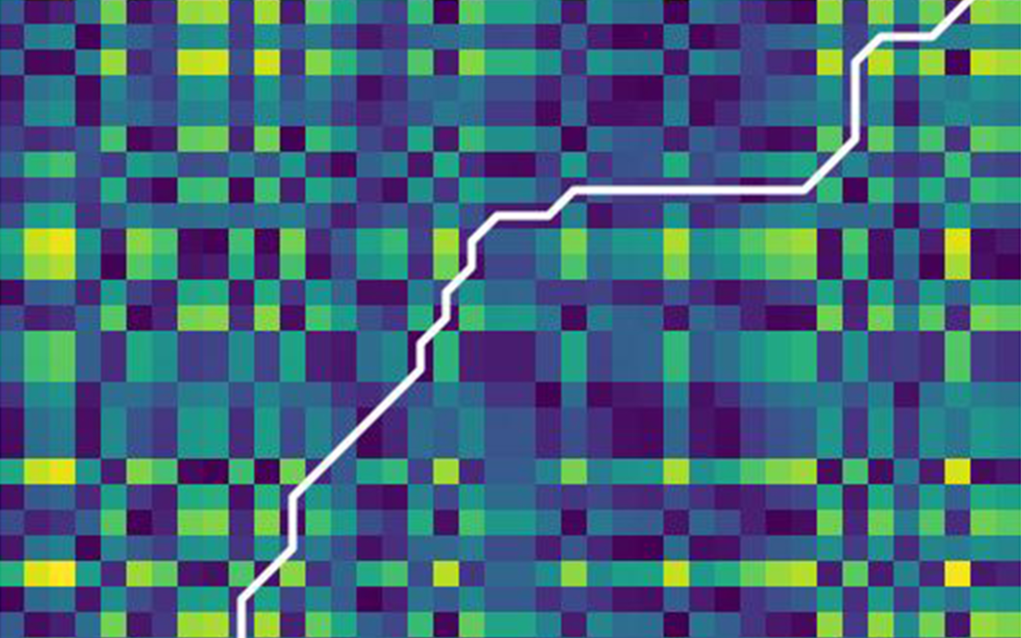
8 Minuten
Something about the aesthetic background
First of all, I would like to address the appeal that the transformations of the designs and working with loops represent for me in this context: The harmony of development and variation within a procedural time process, which ultimately leads to new appearances and thus - across a temporal continuum - contributes to the intensification of perception, lends a striking character to the structures created with the help of loops. The fact that with loops the introduction and introduction of the unexpected into the ongoing forms and processes can be reduced to a minimum without impairing the aesthetic appeal is something that minimal artists, for example, knew how to use very effectively.
The emergence of a diverse whole from the same core - comparable to biological evolution, in which ongoing life develops through gradual changes and new things emerge from the variation of original forms - seems to me both appealing and utopian in the context of artistic creation. After all, persistent adherence to an aesthetic dictated by loops can cause the willingness to perceive to fade in the same way that it has been sharpened.
My search for methods and forms of dealing with loops and their generation in order to unite variations, transitions and transformations between tonal contexts with the rigidity of structures began naively in my earlier instrumental works - mostly purely empirically and without a theoretical or systematic approach.
These early, purely empirical musical transformations lacked a universal, instrumentation-agnostic solution strategy that would have made it possible to apply the methods not only to instrumental music, but also to algorithmic electronic music. My first reaction was to program the same empirically developed manual processes for electronic music, until I noticed the conceptual parallels between my goal, my methodology and those of "dynamic programming", in particular Dynamic Time Warping. Before I go into a summary of this algorithm, however, I would first like to describe the problem of musical transitions in more detail.
The problem of the transition and the search for similarity
Creating a transition means building a bridge between two sides within a certain period of time. In this context, I would like to focus primarily on transitions between sound sequences. Specifically, my article will deal with the transition of the tonal characteristics of a temporally ordered sound sequence.
In doing so, I consider a sound as a multidimensional entity, with each dimension representing a different characteristic of the individual sound: Duration, pitch, intensity and geographical localization are some commonly known dimensions. For digitally synthesized sounds, however, the list can be extended to include all properties relevant to the synthesis. In the simplest case, it is a one-dimensionally defined entity - for example, if we only consider the duration of the sounds for the transition. Trivially, a transition would be created here by interpolating (in the simplest case with the same length of both sequences) between the durations of the individual sounds with the same index.
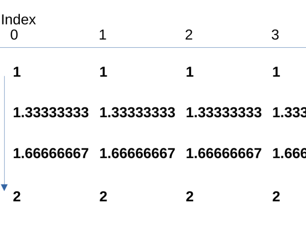
Such a case is shown below, where a linear transition between the 1-dimensional elements of two 4-element sequences has been created over 4 steps. This is a transition from durations (e.g. calculated in seconds) [1, 1, 1, 1] to [2, 2, 2, 2], which represents a ritardando (the frequencies here remain constant and were manually set to 330, 440, 550, 660 Hz):
It is still clear if we increase the number of dimensions per sound from 1 to 2 with the same sequence length. In the following example, I include the frequencies in the transition process and thus expand the dimensions of each entity to two: duration and frequency.
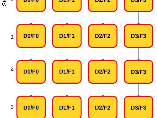
The initial sequence here consists of tones with the durations [1, 1, 1, 1] and frequencies [330, 440, 550, 660] Hertz, while the terminal sequence comprises tones with the durations [2, 2, 2, 2] and frequencies [220, 400, 550, 770] Hertz. As in the previous example, the sound elements are assigned to each other in a straightforward manner: from each index in sequence 1 to the same index in sequence 2 via the specified number of steps (here 4):
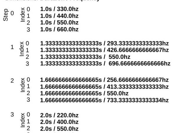
The reason for this simple assignment of the elements lies in the marginal changes in the dimensions between the start and target sequences, which do not affect the relationship between the elements. The sequences of the 4-step transition can therefore be represented as follows:
These are examples where one might think that a simple index-based interpolation between the sequences is sufficient - and in these specific cases it is! However, as soon as the number of sounds in the sequences varies or the differences in the respective dimensions increase, this method is no longer sufficient. Further measures are required to determine the association of the sounds between the sequences (if this association is not to be random).
This is where the calculation of similarities between sounds (viewed as n-dimensional data points) comes into play. Using Dynamic Time Warping, we can use the Euclidean distance between dimensions (the simplest and most common distance metric) to determine an optimal association between elements - even for non-uniform sequences.
Based on the calculation of the distances between the sound dimensions using the Euclidean distance metric, the closer the values of the respective dimensions are to each other, the more similar the sounds are to each other.
What is Dynamic Time Warping?
In the following part, I summarize the dynamic time warping algorithm. More detailed descriptions can be found in the paper by Hiroaki Sakoe and Seibi Chiba (Dynamic Programming Algorithm Optimization for Spoken Word Recognition, IEEE Transactions on Acoustics, Speech and Signal Processing, Vol. ASSP-26, No.1, February 1978) or on the Internet.
The optimization problem
Dynamic Time Warping (DTW) is a method for measuring the similarity between two temporal sequences that may differ in speed and whose elements are located in the same N-dimensional space. It is often used in areas such as speech recognition, gesture recognition and time series analysis. The goal of DTW is to find an optimal alignment between two sequences by distorting the time axis of the sequences so that the distance between them is minimized.
As an example, consider the two time series x = (x0, ....,xn-1) and y = (y0, ....,ym-1) with the respective lengths n and m. The DTW between the sequences x and y is formulated as:

where the alignment path is π = [π0, ...,πk] with the following properties:
1. it is a list with index pairs πk = (ik, jk) where 0 ≤ ik < n and 0 ≤ jk< m
2. π0 = (0, 0) and πk = (n-1, m-1)
3. where k > 0, πk = (ik, jk) is related to πk-1 = (ik-1, jk-1) as follows:
- ik-1 ≤ ik ≤ ik-1 + 1
- jk-1 ≤ jk ≤ jk-1 + 1
The alignment path is a temporal alignment of the two time series x and y so that their distance to each other (often the Euclidean distance) is the smallest.
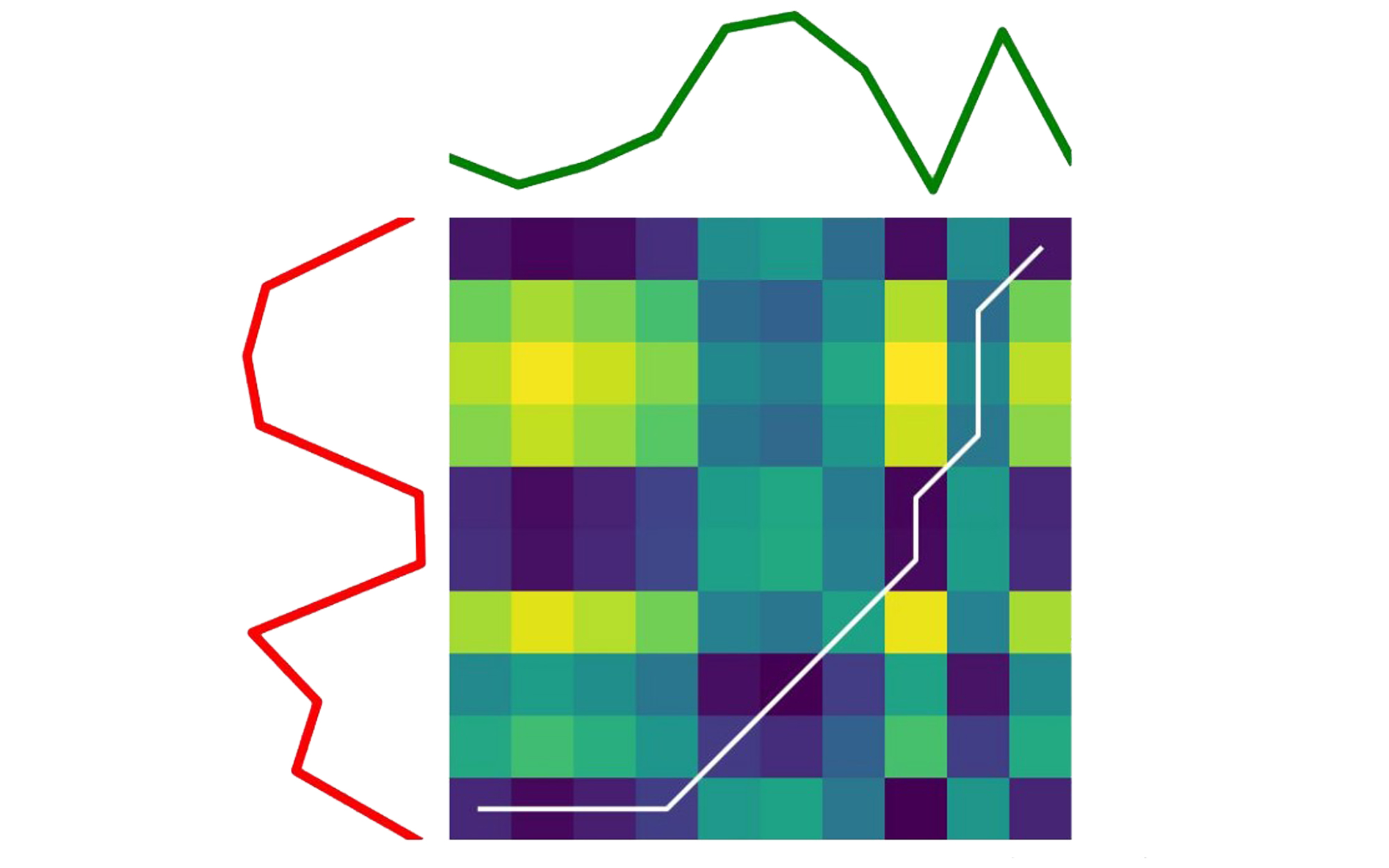
Such an alignment path is shown in the following graphics for two time series with the same size of 10 elements (y-axis: red line, x-axis: green line) with the white line. The white line draws the optimal (shortest) path between the two series on a 10x10 distance matrix, which is shown here as a "heat map". The following applies on the map: The "yellower" the possible step (the individual squares), the greater the distance between the respective elements of the x and y sequences. The optimum path runs from the first element comparison (bottom left, with the clues 0, 0) to the last (top right, with the clues 9, 9) through the "coldest" squares (smallest distance):
The alignment path of two identical sequences is diagonal and straight:
Die Kostenmatrix und der optimale Ausrichtungspfad (weiße Linie) für eine einzelne Zeitreihe.
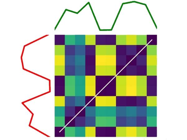
The alignment path of a sequence with its own backward form runs as a symmetrical diagonal line:
Die Kostenmatrix und der optimale Ausrichtungspfad (weiße Linie) für eine Zeitreihe (rot) und ihre umgekehrte Form (grün).
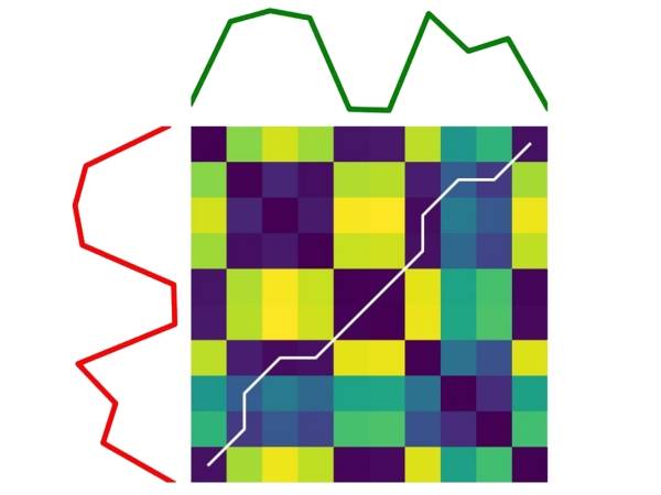
The alignment path of two different sequences:
Die Kostenmatrix und der optimale Ausrichtungspfad (weiße Linie) für zwei verschiedene Zeitreihen.
Sound examples
One could define the alignment path in DTW as the result of finding the optimal closest path between two time series of potentially different durations.
By identifying the most similar pairs of data points between the two sequences, DTW enables an efficient bridging of these correspondences, creating a seamless transition between the time series. Although in most practical applications of DTW the alignment path is primarily used to calculate a similarity value (and is rarely used directly), from an artistic perspective it proves to be a useful tool - e.g. for the stepwise metamorphosis of sound sequences.
As described in the last part illustrating DTW, the raw alignment path can contain one or more mappings between data points. An example path could have the following form: (0,0), (0,1), (1,1), (2,2), (3,2).
Or in visual representation:
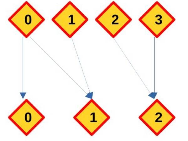
Here, the first data point of the source sequence is assigned to the first two points of the target sequence, while the last two points of the source sequence are mapped to the last point of the target sequence. However, since this path contains redundancies that were not present in the original sequences (multiple links of the same data points), it must be reworked in order to maintain the structural integrity of the original sequences. To do this, I decide between redundant links in favor of the one with the higher similarity value.
Below are two sound examples produced using the alignment path.
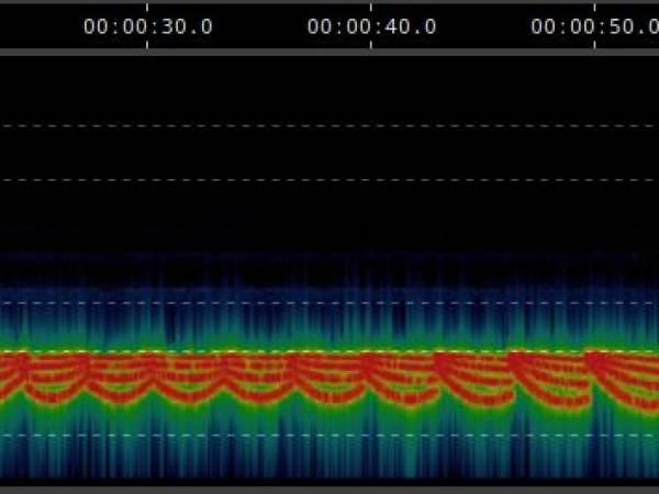
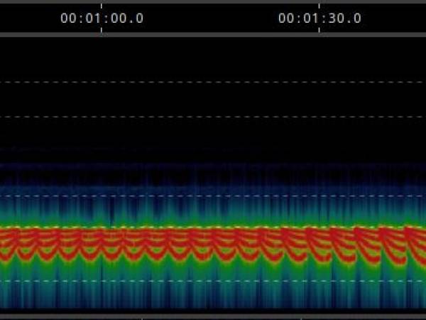
Example 1: A transition between two sequences:
- Source sequence: Four ascending frequency lines with different start frequencies but a common end frequency.
- Target sequence: The reverse output sequence - four frequency lines with identical start frequencies that diverge from the original start frequencies of the output sequence.
Defined parameters are: Duration and frequency of the sounds. It is possible to specify the number of transition steps (start and end state included). For example, a 4-step transition includes 1. initial state, 2. first intermediate step, 3. second intermediate step and 4. target state.
The implementations listed below demonstrate the transition in 6, 12, 25 and finally 50 steps, whereby more steps mean slower changes and thus a smoothing of the transition:
Transition in 6 steps
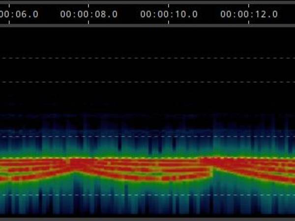
Transition in 12 Stufen
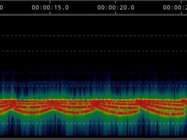
Transition in 25 Stufen
Transition in 50 Stufen
Example 2: Sequence of transitions:
1. from the children's song "Hänschen klein" to "Alle meine Entchen" in 17 steps:
2. an extended path also integrates the opening theme from Steve Reich's "Piano Phase":
- "Hänschen klein" → "Piano Phase" motif (in 20 steps)
- "Piano Phase" → "All my little ducklings" (in 15 steps)
Musical use
The appeal of this method lies in its independence from musical stylistic characteristics: The algorithm processes sound sequences independently of genre-specific characteristics. This opens up a broad field of experimentation for "transitional music", in which even stylistically contrasting sound sequences can flow into one another. In the following section, I present a short work of my own whose sound materials were obtained from transitions created with the help of DTW.
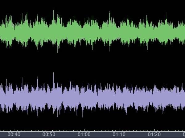
Transition Studies (2024/25, first movement)
"Transition Studies" is a four-channel work consisting of three short pieces. The first 2-minute movement consists of a single continuous, uninterrupted transition between two sound gestures that can be heard at the beginning and end of the piece. In addition to temporal variations of the two initial and final sound sequences, the subject of this transition in this movement is also a modulation in the playback speed of the samples used, as well as a transition in the geographical location of the sounds (which sound from which loudspeaker). It is therefore a three-dimensional transition: duration, modulation factor and localization.
The movement is associated with brutalist architecture through its raw sound materiality and rough formal progression.
Below is a stereo mix of this movement.

Amir Teymuri
Amir Teymuri studied composition, piano and music informatics at the University of Tehran, the Hochschule für Musik Freiburg, the Hochschule für Musik und Darstellende Kunst Frankfurt am Main and at the Institute for Music Informatics and Musicology at the Hochschule für Musik Karlsruhe. In 2004, he was honored at the First National Biennial of New Music at the University of Tehran. In 2015, he was a fellow of the Akademie der Künste (AdK Berlin) and artist-in-residence at the Center for Art and Urbanistics (ZK/U Berlin). In addition to his work as a freelance composer, he is currently a lecturer at the University of Music and Performing Arts Munich and at the Institute for Music Informatics in Karlsruhe.
Article topics
Article translations are machine translated and proofread.
Artikel von Amir Teymuri
// Similar articles